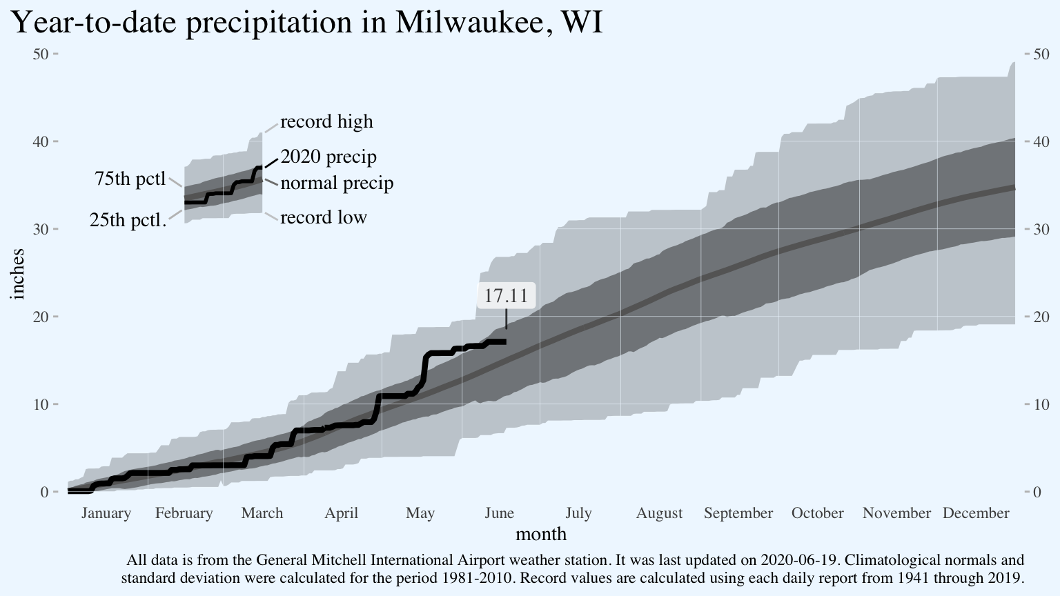
How to build a Tufte-style weather graph in R using ggplot2
This notebook contains all the code needed to create this graph.
Background
I have been greatly influenced by Edward Tufte’s work on data visualization. When I was learning R, Bradley Boehmke’s replication of Tufte’s daily temperature graph was a great help in getting a better grasp of the R packages dplyr, tidyr, and ggplot2. Quite a bit has changed in the tidyverse since Boehmke wrote that post in 2015. In this document, I aim to provide an updated demonstration of some tidyverse tools for data manipulation and visualization as well as some examples of how to pull data from the National Oceanic and Atmospheric Agency’s FTP server.
Unlike Boehmke’s project, this graph does not directly replicate anything Edward Tufte has made. Instead I try to apply some of his principles of design to a different dataset–cumulative annual precipitation. In doing so, I made a set of aesthetic choices in making this graph which you may disagree with. Future me may disagree with them too, but by documenting the process of creating these graph in detail I hope I’ll give you some new ideas on how to use ggplot2’s nearly infinite options to tweak graphs to your heart’s content.
Data
I’ve pre-processed the data needed for this plot, and you can download it using the code below. If you want to make this graph for a different weather station, please refer to this post for a demonstration of how to retrieve and process this data from NOAA.
library(tidyverse)

all.precip.data <- read_csv("https://johndjohnson.info/files/MilwaukeePrecipitationData2020.csv")
Building the plot
Before beginning, create some helpful vectors for the x-axis lines and labels.
leapyear.month.breaks <- all.precip.data %>%
  group_by(month) %>%
  filter(dayofleapyear == min(dayofleapyear)) %>%
  pull(dayofleapyear)
leapyear.month.mids <- all.precip.data %>%
  group_by(month) %>%
  summarise(dayofleapyear = median(dayofleapyear)) %>%
  pull(dayofleapyear)
p <- ggplot(all.precip.data) +
ggthemes::theme_tufte() +
theme(plot.background = element_rect(fill = "aliceblue",
colour = "aliceblue"))
p
Begin adding the data. First, I plot the record values as a ribbon. The alpha value controls the opacity of the ribbon. I could also control the relative darkness of the ribbons by assigning them different colors, but in this case setting the transparency was a good shortcut.
p <- p +
  geom_ribbon(aes(x = dayofleapyear,
                  ymin = low_cum_precip,
                  ymax = max_cum_precip),
              alpha = 0.25)
p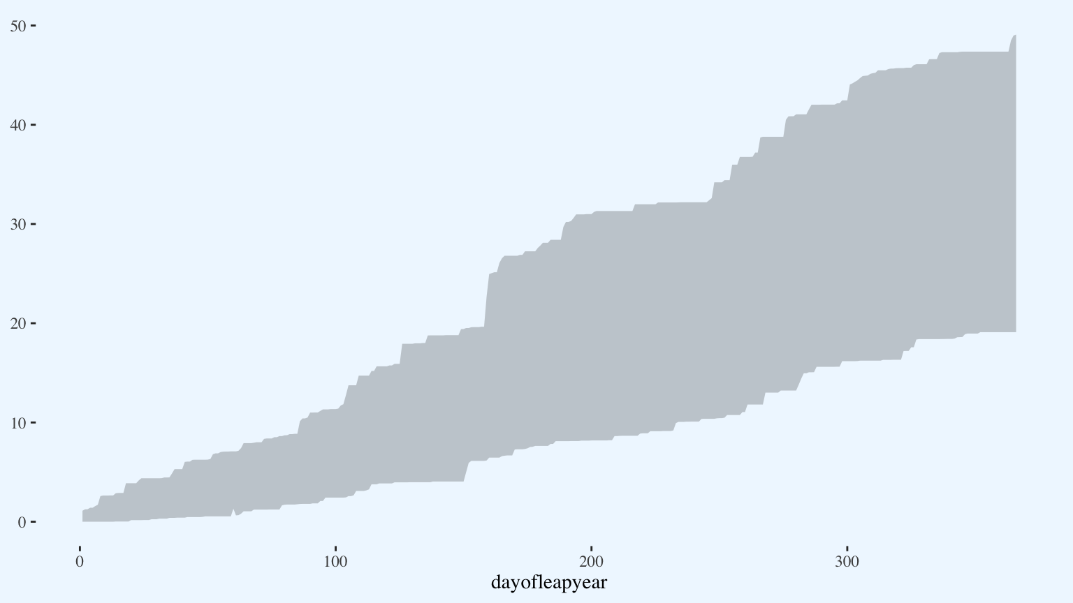
Add a ribbon for the standard deviation.
p <- p +
  geom_ribbon(aes(x = dayofleapyear,
                  ymin = (normal_precip - ytd_precip_sd),
                  ymax = (normal_precip + ytd_precip_sd)),
              alpha = 0.5)
p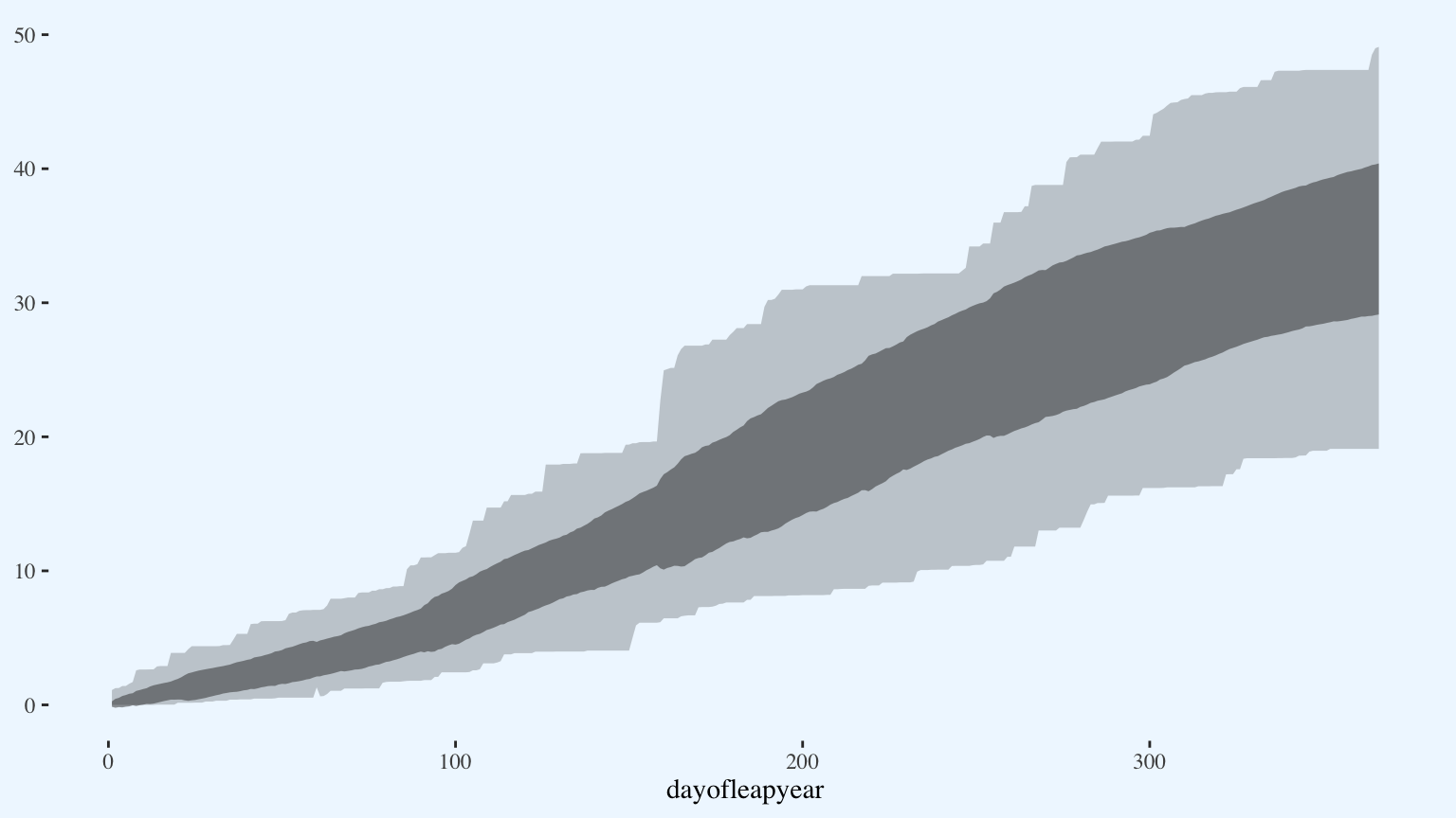
Add a line for the climatological normal value.
p <- p +
  geom_line(aes(x = dayofleapyear,
                y = normal_precip),
            color = "gray40",
            size = 1.5)
p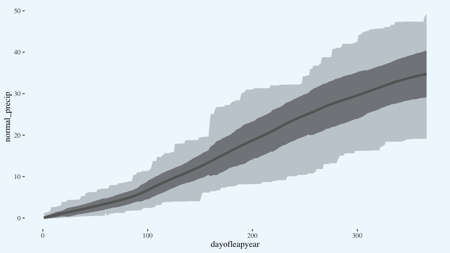
Add this year’s data.
p <- p +
  geom_line(aes(x = dayofleapyear,
                y = cum_precip_2020),
            size = 1.5)
p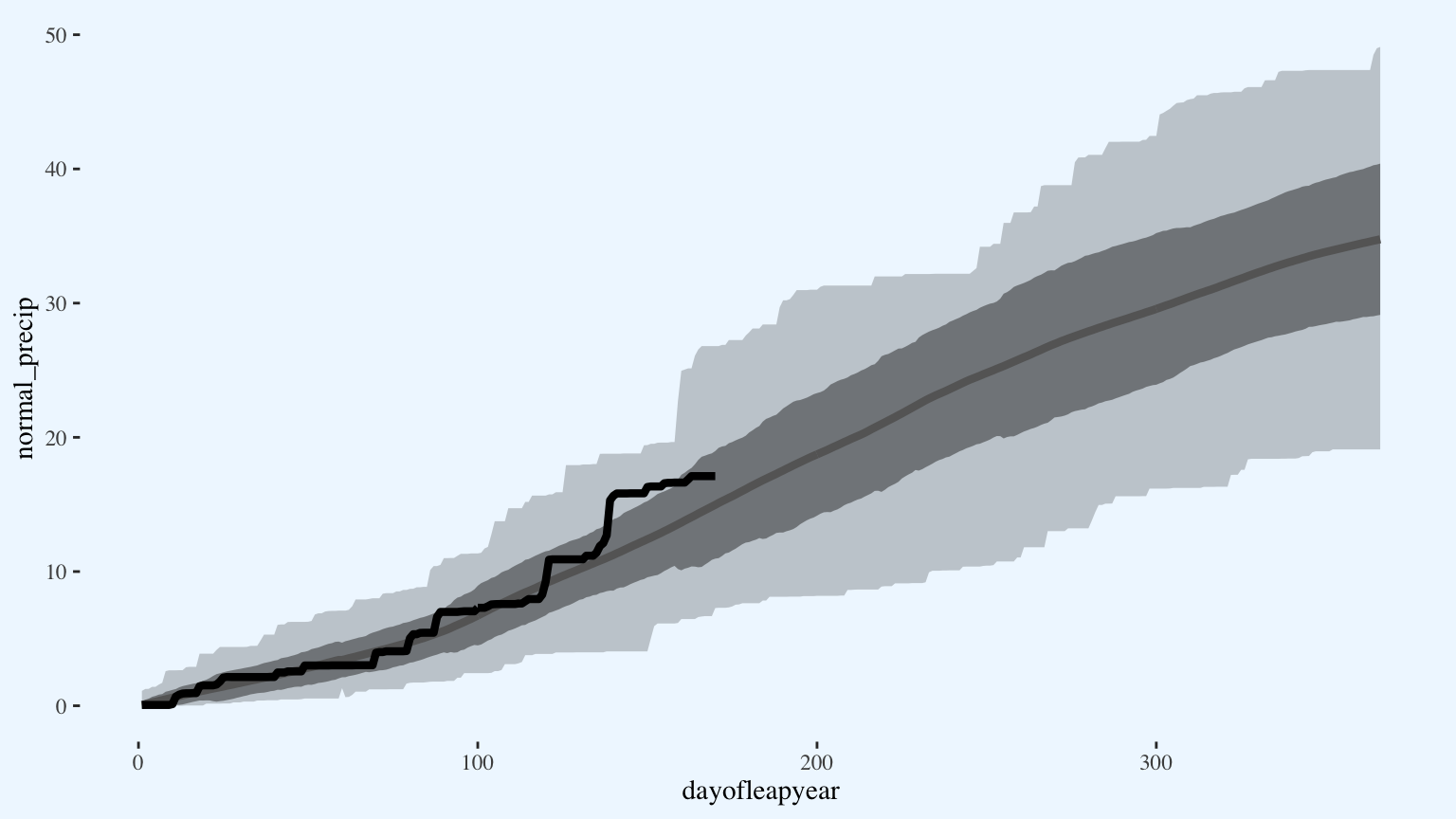
Because this graph has so many custom pieces, it needs a custom legend. I’ll use the empty space in the upper left-hand corner of the graph.
legend.data <- all.precip.data %>%
  filter(month == 3) %>%
  # move the data further back on the x-axis
  mutate(dayofleapyear = dayofleapyear - 15) %>%
  # move the data up on the y-axis
  mutate(normal_precip = normal_precip + 30,
         max_cum_precip = max_cum_precip + 30,
         low_cum_precip = low_cum_precip + 30,
         cum_precip_2020 = cum_precip_2020 + 30)

p <- p +
  geom_ribbon(data = legend.data, aes(x = dayofleapyear,
                                      ymin = low_cum_precip,
                                      ymax = max_cum_precip),
              alpha = 0.25) +
  geom_ribbon(data = legend.data, aes(x = dayofleapyear,
                                      ymin = (normal_precip - ytd_precip_sd),
                                      ymax = (normal_precip + ytd_precip_sd)),
              alpha = 0.5) +
  geom_line(data = legend.data, aes(x = dayofleapyear,
                                    y = normal_precip),
            color = "gray40",
            size = 1.5) +
  geom_line(data = legend.data, aes(x = dayofleapyear,
                                    y = cum_precip_2020),
            size = 1)
p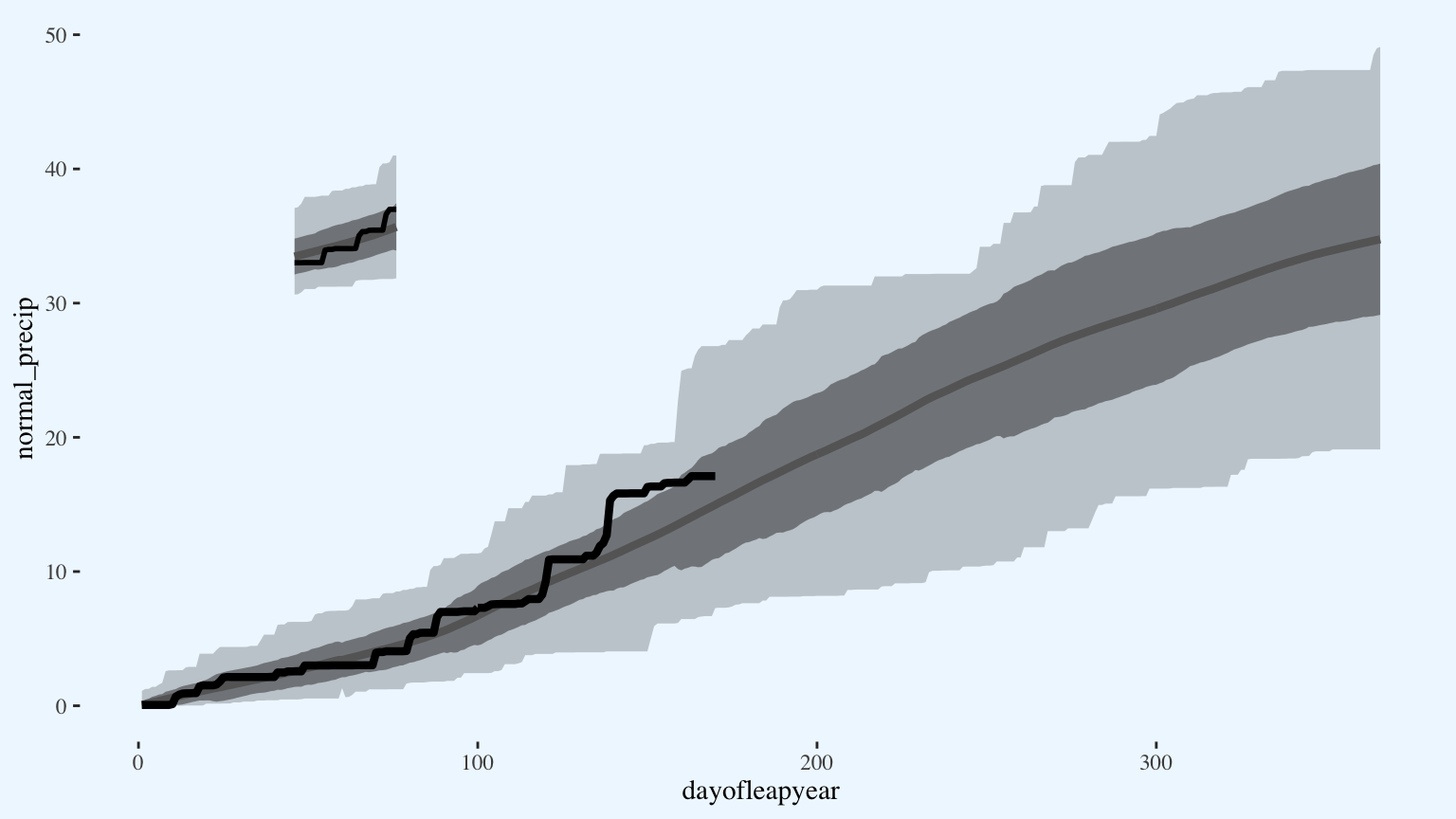
Add the gridlines. By inserting custom gridlines on top of the data and the same color as the background, I make the grid only appear on top of the data as negative space.
p <- p +
  geom_vline(xintercept = leapyear.month.breaks,
             color = "aliceblue",
             size = 0.1) +
  geom_hline(yintercept = c(0,10,20,30,40,50),
             color = "aliceblue",
             size = 0.1)
p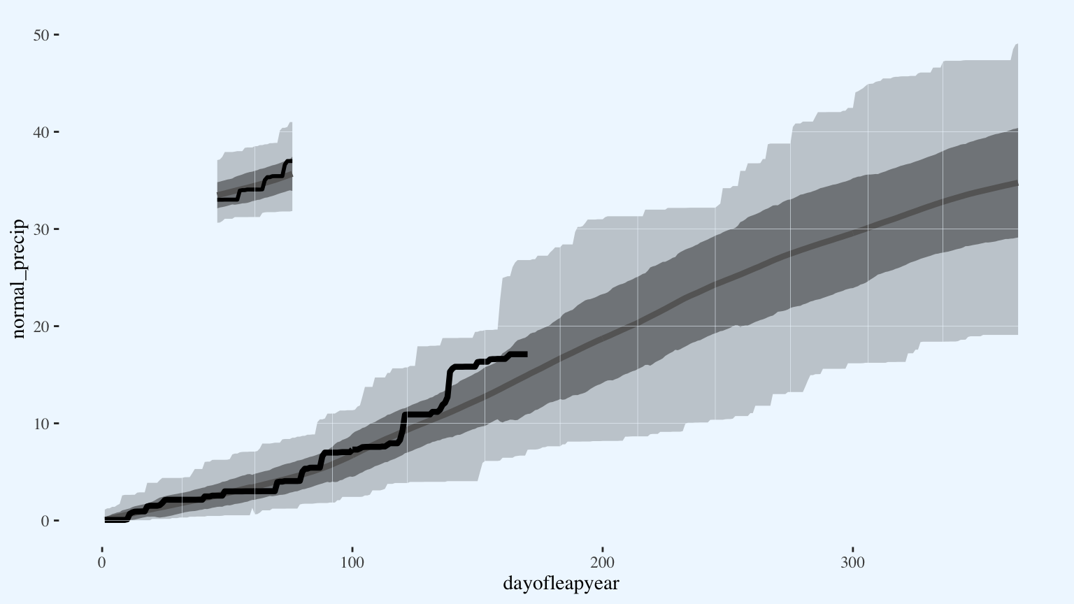
Add the legend annotations on top of the gridlines. There are some on-the-fly ways to automate labeling data points (e.g. the ggrepel package), but for a polished graph there isn’t a subsitute for doing it by hand.
p <- p +
  annotate("segment", x = 77, xend = 82,
           y = legend.data$max_cum_precip[legend.data$dayofleapyear == 76],
           yend = 42, color = "gray", alpha = 0.75) +
  annotate("text", x = 83, y = 42, family = "serif",
           label = "record high", hjust = 0, vjust = 0.25) +
  annotate("segment", x = 77, xend = 82,
           y = legend.data$cum_precip_2020[legend.data$dayofleapyear == 76],
           yend = 38, color = "black") +
  annotate("text", x = 83, y = 38, family = "serif",
           label = "2020 precip", hjust = 0, vjust = 0.25) +
  annotate("segment", x = 77, xend = 82,
           y = legend.data$normal_precip[legend.data$dayofleapyear == 76],
           yend = 35, color = "gray50") +
  annotate("text", x = 83, y = 35, family = "serif",
           label = "normal precip", hjust = 0, vjust = 0.25) +
  annotate("segment", x = 77, xend = 82,
           y = legend.data$low_cum_precip[legend.data$dayofleapyear == 76],
           yend = 31, color = "gray", alpha = 0.75) +
  annotate("text", x = 83, y = 31, family = "serif",
           label = "record low", hjust = 0, vjust = 0.25) +
  annotate("segment", x = 45, xend = 40,
           y = legend.data$normal_precip[legend.data$dayofleapyear == 46] -
             legend.data$ytd_precip_sd[legend.data$dayofleapyear == 46],
           yend = (legend.data$normal_precip[legend.data$dayofleapyear == 46] -
                     legend.data$ytd_precip_sd[legend.data$dayofleapyear == 46]) - 1,
           color = "gray75") +
  annotate("text", x = 39,
           y = (legend.data$normal_precip[legend.data$dayofleapyear == 46] -
                  legend.data$ytd_precip_sd[legend.data$dayofleapyear == 46]) - 1,
           label = "25th pctl.", family = "serif", hjust = 1) +
  annotate("segment", x = 45, xend = 40,
           y = legend.data$normal_precip[legend.data$dayofleapyear == 46] +
             legend.data$ytd_precip_sd[legend.data$dayofleapyear == 46],
           yend = (legend.data$normal_precip[legend.data$dayofleapyear == 46] +
                     legend.data$ytd_precip_sd[legend.data$dayofleapyear == 46]) + 1,
           color = "gray75") +
  annotate("text", x = 39,
           y = (legend.data$normal_precip[legend.data$dayofleapyear == 46] +
                  legend.data$ytd_precip_sd[legend.data$dayofleapyear == 46]) + 1,
           label = "75th pctl", family = "serif", hjust = 1)
p
Edit the axis text.
p <- p +
  scale_x_continuous(breaks = leapyear.month.mids,
                     labels = month.name,
                     name = "month",
                     expand = expansion(0.01)) +
  scale_y_continuous(breaks = c(0,10,20,30,40,50),
                     name = "inches",
                     sec.axis = dup_axis(name = NULL),
                     expand = expansion(0.01))
p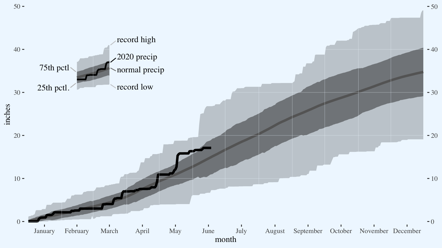
Add the explanatory text. I find it’s often easier to assign long labels to object outside the ggplot object, then include it in the graph’s code using stringr::str_wrap.
last.date.updated <- "2020-06-19"
caption.text <- paste("All data is from the General Mitchell International Airport weather station. ",
                      "It was last updated on 2020-06-19.",
                      "Climatological normals and standard deviation were calculated for the period 1981-2010. ",
                      "Record values are calculated using each daily report from 1941 through 2019.")
p <- p +
  labs(title = "Year-to-date precipitation in Milwaukee, WI",
       caption = str_wrap(caption.text, 145))
p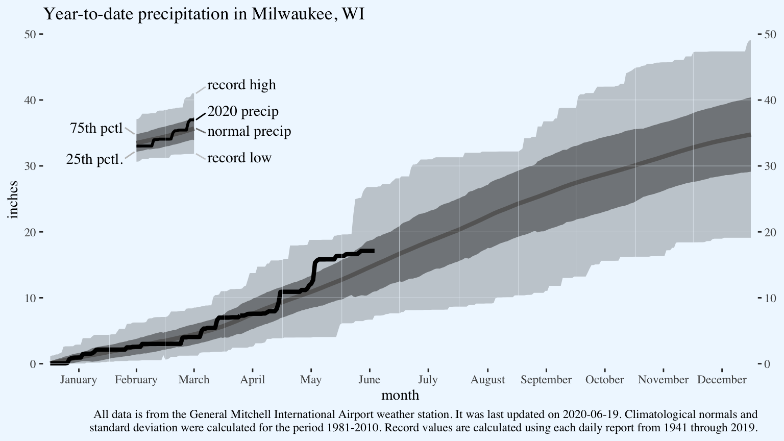
Add a text label for the most recent data point. The package ggrepel helpfully adds some padding to the point. It’s not necessary in this case since I’m only labelling a single point, but it is extremely helpful when you have multiple points and don’t want to specify the label position for each one.
The bit of code data = function(x){...} subsets the data.frame from way back in the original ggplot line for the last day of available 2020 data.
p <- p +
  ggrepel::geom_label_repel(data = function(x){
    x %>%
      filter(!is.na(cum_precip_2020)) %>%
      filter(dayofleapyear == max(dayofleapyear))
  },
  aes(x = dayofleapyear,
      y = cum_precip_2020,
      label = cum_precip_2020),
  family = "serif",
  alpha = 0.75,
  point.padding = 1,
  nudge_y = 1,
  label.size = 0)
p
Finally, tweak the appearance of the axes and change the alignment and size of the plot’s title.
p <- p +
  theme(axis.ticks.x = element_blank(),
        plot.title.position = "plot",
        axis.ticks.y = element_line(color = "gray",
                                    size = 0.5),
        plot.title = element_text(size = 18))
p