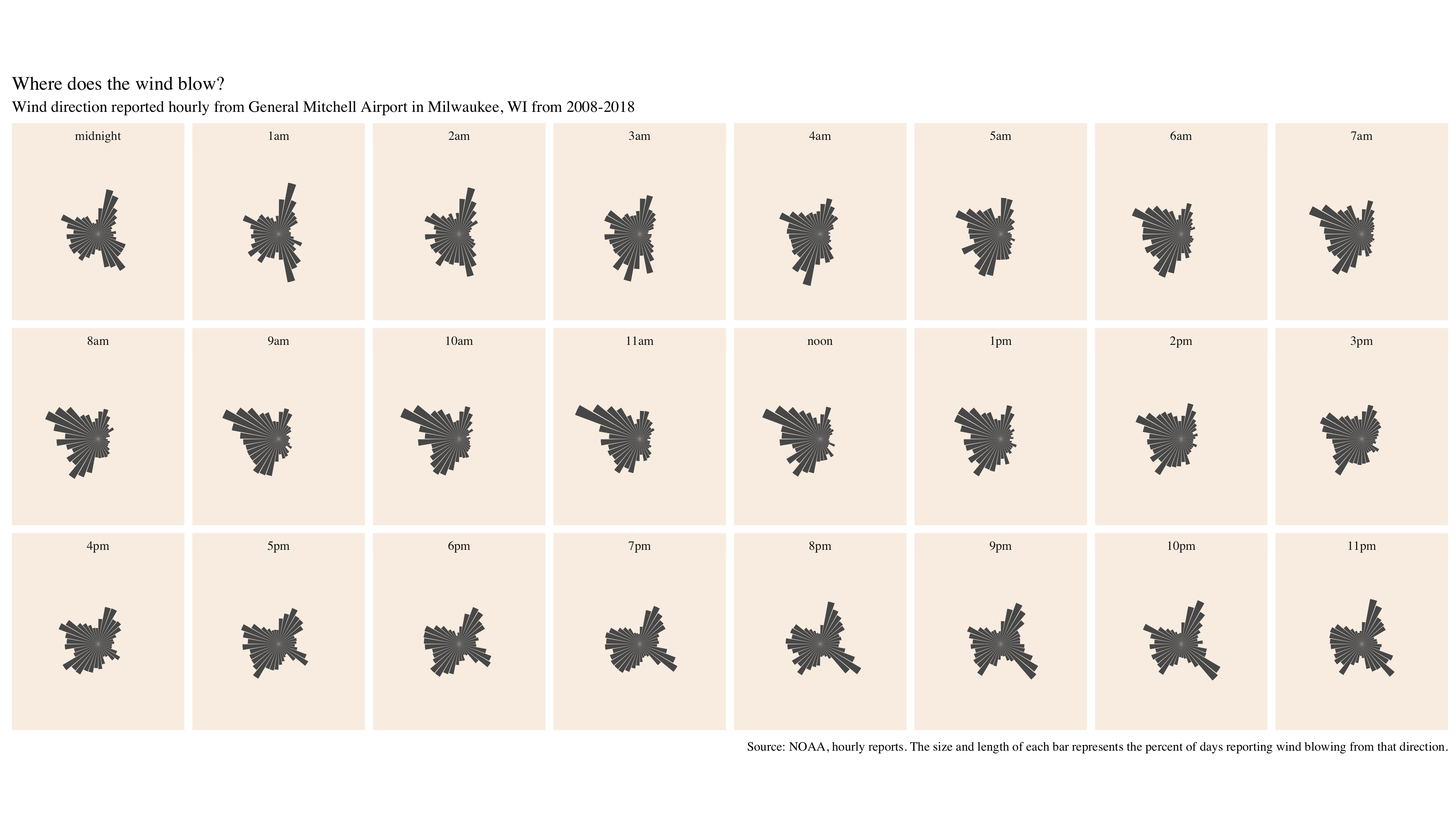
The wind in Milwaukee is strongly affected by Lake Michigan. When the sun sets and land temperatures cool, the wind often blows from the east. During the day the land heats up and the reverse happens.

You can see an amazing live visualization of the wind here

I wanted to see how the wind varies by time of day, so I made this series of small multiples using hourly weather records from NOAA. To download a full size version click here.

You can make the graph yourself using the following code.

library(tidyverse)
library(labelled)

# you can make the range of years anything you want
years <- 2008:2018
d.years <- list()


for(i in seq_along(years)){
  d <- read_csv(paste0("https://www.ncei.noaa.gov/data/global-hourly/access/",
                       years[i], "/72640014839.csv"),
                col_types = cols(.default = "c"))
  d <- d %>%
    select(STATION, DATE, WND) %>%
    separate(col = "WND", sep = ",", convert = F,
             into = c("angle", "angle_code", "type_code", "speed",
                      "speed_code")) %>%
    mutate(speed = replace(speed, speed == 9999, NA),
           angle = replace(angle, angle == 999, NA)) %>%
    separate(col = "DATE", into = c("date","time"), sep = "T") %>%
    separate(col = "time", sep = ":", into = c("hour","minute","second"),
             remove = F, convert = F) %>%
    select(-second)
  
  d.years[[i]] <- d
  rm(d)
}

wind <- bind_rows(d.years)

wind2 <- wind %>%
  mutate(angle = as.numeric(as.character(angle)),
         hour = as.numeric(as.character(hour)),
         minute = as.numeric(as.character(minute)))

wind3 <- wind2 %>%
  mutate(hour2 = hour, 
         hour2 = replace(hour2, minute > 30, hour[minute > 30] + 1),
         hour2 = replace(hour2, hour2 == 24, 0),
         category = cut(angle, breaks = c(seq(0, 360, by = 10)))) %>%
  filter(!is.na(angle)) %>%
  group_by(hour2) %>%
  mutate(observations = n()) %>%
  group_by(hour2, category) %>%
  summarise(pct = n()/first(observations)) %>%
  ungroup() %>%
  set_value_labels(hour2 = c("midnight" = 0, "1am" = 1, "2am" = 2, "3am" = 3,
                             "4am" = 4, "5am" = 5, "6am" = 6, "7am" = 7,
                             "8am" = 8, "9am" = 9, "10am" = 10, "11am" = 11,
                             "noon" = 12, "1pm" = 13, "2pm" = 14, "3pm" = 15,
                             "4pm" = 16, "5pm" = 17, "6pm" = 18, "7pm" = 19,
                             "8pm" = 20, "9pm" = 21, "10pm" = 22, "11pm" = 23)) %>%
  mutate(hour2 = to_factor(hour2))


by.hour <- ggplot(wind3, aes(category, pct)) +
  geom_histogram(stat = "identity") +
  coord_polar(theta = "x") +
  facet_wrap(facets = vars(hour2),
             nrow = 3) +
  labs(title = "Where does the wind blow?",
       subtitle = "Wind direction reported hourly from General Mitchell Airport in Milwaukee, WI from 2008-2018",
       caption = paste("Source: NOAA, hourly reports. The size and length of", 
                       "each bar represents the percent of days reporting wind", 
                       "blowing from that direction.")) +
  theme_bw(base_family = "serif") +
  theme(axis.text = element_blank(),
        axis.ticks = element_blank(),
        axis.title = element_blank(),
        panel.grid = element_blank(),
        panel.background = element_rect(fill = "linen"),
        panel.border = element_blank(),
        strip.background = element_rect(fill = "linen",
                                        colour = "linen"))